
Table of contents
2.2.1 Reflectance and emittance spectra
2.2.2 Spectral coverage of free and low-cost satellite image data
Introduction
Geologists are well served by readily available digital remote sensing data covering a variety of electromagnetic (EM) wavelengths. The data have spatial resolving power from <10 cm in the case of images captured from various aerial platforms (e.g. aircraft, drones, kites etc.) covering a few km2 on the ground, to those comprising pixels that represent patches on the ground 250 m across from the super-synoptic Moderate Resolution Imaging Spectroradiometer (MODIS aboard the NASA Terra and Aqua satellites) for areas 2300 km across.
The significance of being able to use image data from a range of wavelengths stems from the contrasting ways in which different surface materials reflect and emit electromagnetic radiation, over that range. Apart from imaging radar, most remote-sensing depends on either solar radiation that illuminates the surface during daylight hours or on radiation that Earth materials emit through having been heated by the Sun. Radar imaging depends on artificially illuminating the surface with pulses of microwave radiation at wavelength to which the atmosphere, including clouds, is to all intents transparent. Radar pulses interact with surface materials so that a proportion of the radar energy returns to a detector. In the case of solar radiation and that emitted by the surface, the absorbent properties of the atmosphere, mainly due to water vapour, oxygen and carbon dioxide, block some parts of the full EM wavelength range while allowing other ranges to pass more or less unhindered. That is, under cloud-free conditions.
A summary of some theoretical aspects of EM radiation helps underpin the practicalities of remote sensing
The range of wavelengths and the power of radiation at different wavelengths emitted by the Sun and the Earth’s surface depend on the absolute temperature of the source: ~6000 K for the solar surface and ~300 K for that of the Earth (Figure 2.1).
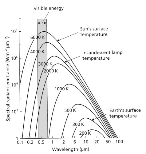
The area beneath each curve in Figure 2.1 represents total power emitted (H) at each temperature. This is proportional to the fourth power of the temperature (T), expressed by the Stefan-Boltzmann Law:
H = σT4
where σ is the Stefan-Boltzmann constant (5.7 x 10⁻⁸ Wm2K-4). As the temperature decreases the wavelength of maximum emittance increases according to Wien’s Displacement Law (λmax = 2898/T mm), while the range of wavelengths and the total emittance decrease. So, the range of wavelengths emitted by a blackbody at the average temperature of the Earth itself is restricted to the mid-infrared between 3 to 50 μm with a peak around 10 μm.
A blackbody at the surface temperature of the Sun is capable of emitting radiation in wavelengths from <0.1 to 100 μm, peaking in the humanly visible range at around 0.5 μm: approximately the wavelength of green light. The concept of a blackbody is theoretical, real surfaces only approximating the properties shown in Figure 2.1. The Sun’s irradiation curves for the near vacuum of outer space and at the base of the atmosphere are shown in Figure 2.2. Clearly, not all wavelengths in solar radiation pass through the atmosphere to the same extent.
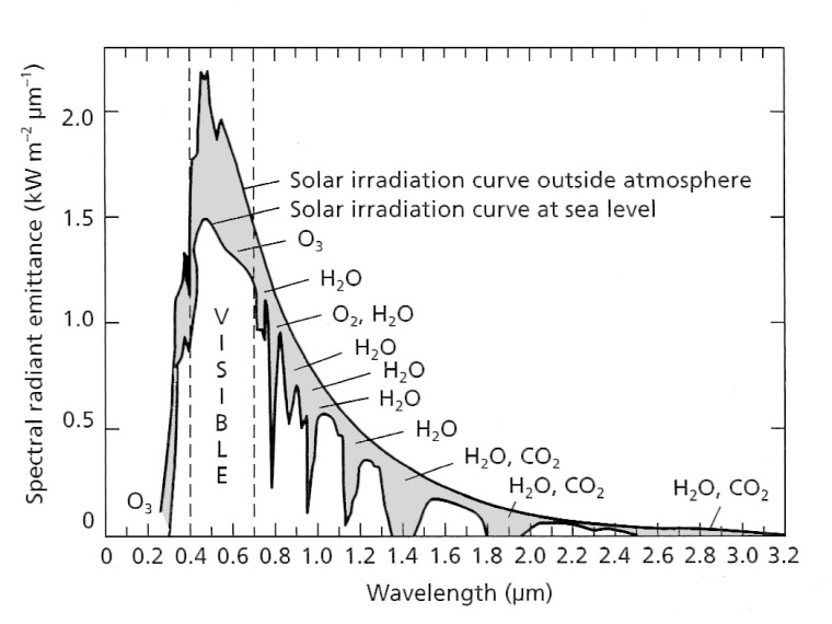
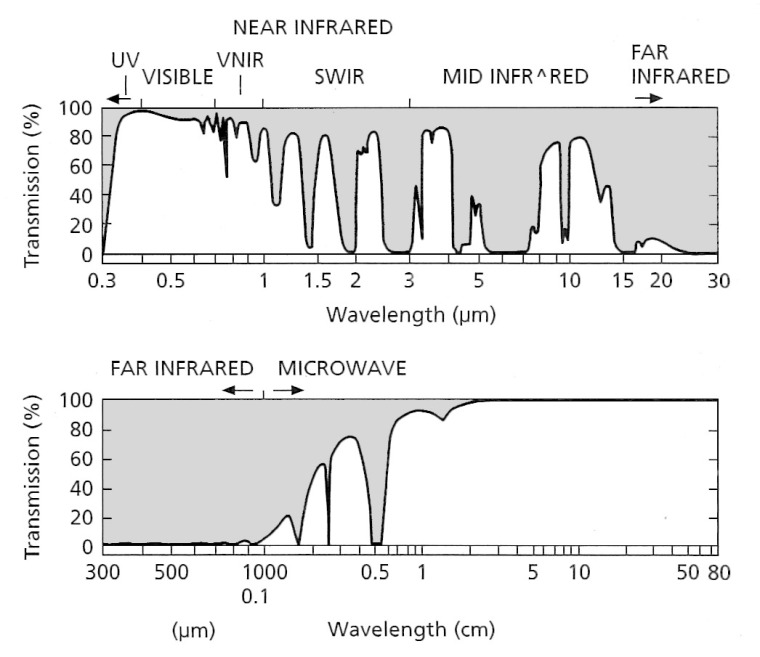
Absorption by various atmospheric gases occurs throughout the EM spectrum, which restricts remote sensing to those wavelength ranges that are least affected by radiation having to pass through air: so-called atmospheric ‘windows’ (Figure 2.3).
A final effect of the atmosphere that is important in remote sensing is the way that gas molecules, aerosols and dust scatter radiation. Scattering disperses radiation in random directions to produce a diffuse effect. Atmospheric scattering is dominated by two processes: that due to molecules of oxygen (O2) and nitrogen (N2) that are smaller than the shortest wavelengths in solar radiation, and by fine aerosols, dust particle and water molecules that are about the same size as wavelengths of visible radiation.
In the first process the degree of scattering is inversely proportional to the fourth power of wavelength. Consequently it mainly affects the blue component of light but has little influence on longer wavelengths; this results in the blue colour of the sky and the way increasingly distant mountains appear progressively more bluish to us. The second kind of scattering affects the longer wavelengths of visible radiation, and results in the redness of sunsets, that are especially vivid when volcanic emissions of dust and sulfuric acid aerosols enter the upper atmosphere.
Radar – originally an acronym derived from radio detection and ranging – exploits the broad microwave region of the EM spectrum from 0.8 to 80 cm (Table 2.1), where the atmosphere is almost transparent to radiation (Figure 2.3). Because of this transparency little power is lost during the passage of microwave radiation through the atmosphere, making it possible to deploy radar imaging devices on orbiting satellites without insuperable demands for electrical power. Relying on artificially generated EM radiation, radar can operate at any time of day or night. Moreover, it also penetrates even dense cloud with little reduction in power: radar is almost an all-weather imaging method. The only likely source of interference is from heavy rain, hail or snowfall. But as you will see later in this chapter, radar data are rarely low-cost and they have a host of peculiarities.
Table 2.1 Divisions in the microwave region employed by radar systems. The letter codes stem from military security measures used during the early development of radar.
| Radar band code | Wavelength (cm) |
| Ka | 0.8-1.1 |
| K | 1.1-1.7 |
| Ku | 1.7-2.4 |
| X | 2.4-3.8 |
| C | 3.8-7.5 |
| S | 7.5-15 |
| L | 15-30 |
| P | 30-100 |
Most images in the reflected and emitted regions are acquired looking vertically downwards, which gives them a map-like quality. The various methods used to capture images of reflected and emitted radiation are outside the scope of this project, and it is unnecessary to be familiar with them here. They are well covered by many textbooks on remote sensing, examples being those in the Useful References section.
Radar imaging is very different from common concept of taking pictures, and a brief explanation will be useful. Radar images are always captured ‘looking’ at an oblique angle towards the surface. The reason for this is that radar images depend on extremely precise measurement of the time taken for microwaves to travel to the target and for a proportion of the microwave radiation to return to the detecting antenna. Rather than bathing the surface continually with a microwave beam, the ‘sideways-looking’ deployment sends very short pulses of radiation, so that emitted and returning energy are not confused at the receiving antenna. Moreover, the radiation used is effectively in the form of a microwave laser, whose remarkable properties make imaging radar possible.
Within the ground area illuminated by a radar pulse, some is slightly ahead of the platforms movement over the Earth, some is behind and only a minor proportion at right angles to the platform’s trajectory. As a result, parts of the returned signal from ahead and behind include a Doppler shift in the microwaves’ wavelength – shorter from the surface ahead of the platform and longer from behind – whereas only returns from 90° to the direction of travel remain at the same wavelength as the emitted microwaves. By allowing the returns to interfere with a reference signal at the same wavelength as the emitted microwaves the ahead- and to-the-rear signals can be distinguished digitally. Effectively, imaging radar therefore ‘looks’ at any point on the surface several times, the signals from ahead, directly to the side and behind being discriminated by the Doppler shift. The further away the surface, the more times it is ‘looked at’ because of the spread of the beam, and that allows the spatial resolution of the resulting image to be independent of distance to the side or range. Exploiting the Doppler shift enables quite low powered radar systems to capture equally detailed images from orbit as they can from an aircraft.
The key to producing these synthetic aperture radar (SAR) images is recording the intensity of returning microwave pulses and the time at which they are received in relation to their time of transmission, which takes the form of a mathematically very complex ‘map’ of the recorded interference patterns. In the earliest systems this information produced an optical hologram recorded on film, through which a laser was projected to ‘correlate’ the interference patterns and thereby create an image of the surface. Digitally recorded SAR images are processed by sophisticated software to the same end.
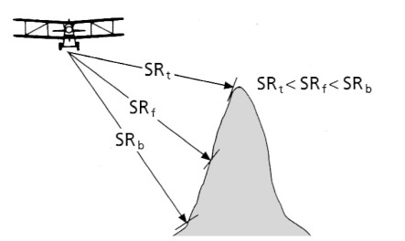
The sideways ‘look’ and recording of intensity and time by radar imaging produces unique geometric distortions. Times represent distances to the surface obliquely to the side of the platform. To convert a radar image to a map-like form requires a correction for this. However, there is still a distortion because the distance is not merely as measured on a map, but depends on the effect of varying topographic elevation on the measured return times from to the surface of the spherical wavefronts of the radar pulses (Figures 2.4 to 2.6). That relationship gives rise to two kinds of distortion: ‘layover’ (Figure 2.4) and foreshortening (Figure 2.5), both shown by the SAR image in Figure 2.6. The distortion of identical topographic features changes as distance from the antenna progressively increases.
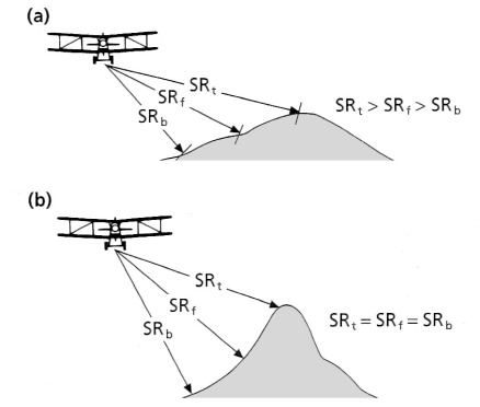

Because they result from active illumination of the surface, radar images also contain shadows that, unlike those on images of reflected solar radiation that are partly illuminated by scattered radiation, are completely black. Distortions and shadows tend to highlight relief far more in radar images than in those of reflected solar and emitted thermal radiation. Consequently they enhance features controlled by geological structure, albeit at the expense of a directional bias produced by the uniform illumination direction.
2.1 Issues of resolution
The term resolution when applied to an image refers in a general way to the amount of spatial detail that it records: a function of the optics of the imaging system and how far the platform is from the scene that is imaged. Most images in use nowadays are digital so the ‘unit’ of resolution is the pixel (short for picture element), most readily understood from the grid-like arrangement of charge-coupled devices (CCDs) used in digital cameras, e.g. a one megapixel camera’s CCD has a million elements arranged in a grid.
There is no real limit to how fine image resolution can be when captured from close to the surface – the device can be moved as close as one wishes. But there is a limit to the resolution of satellite images, which results from turbulence in the atmosphere, expressed by the shimmering of stars on a clear night. It is estimated that atmospheric shimmer limits spatial resolution from orbit to about 15 cm, although sophisticated software that models turbulence is capable of reducing that somewhat in image intelligence circles. At the time of writing (mid-2014) the finest resolution available from commercial remote-sensing satellites is 30 cm for panchromatic (black and white) images from Digital Globe’s WorldView3 system (Appendix 1). Such publically available precision followed progressive relaxation of US government regulations banning sales of high-resolution images except to ‘Government customers and specifically designated allies’. To throw this into sharp perspective, when the Landsat-5 Thematic Mapper went into orbit in 1984, release to the public of its 30 m resolution data was, for a while, regarded as being against US national interests. Landsat TM’s potential commercial use soon over-rode that perhaps slightly paranoid attitude. There were also diplomatic issues, since any country not possessing top-of-the-range remote sensing satellites might fear for the security of their secret installations and vital infrastructure. A measure of the degree to which that is now ignored is the free availability for at least a proportion of every country of <1 m resolution natural colour satellite images on Google Earth, on which even pedestrians can be made out – though not recognised.
The other aspect of spatial resolution relates to the resolving power of the human eye and visual cortex. That depends on the number and distribution of individual detectors on the retina. These are of two types: rods that are most sensitive to green and blue light under bright and dim conditions respectively, and three types of cones sensitive to what we perceive as red, green and blue light that endow us with full colour vision. However, rods vastly outnumber cones on the retina (Figure 2.7).
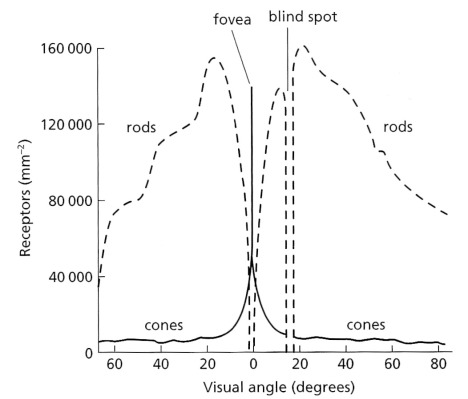
As a result of the predominance of rods over cones the degree to which we resolve spatial detail depends to a large extent on the contrast within an image, increased contrast being an increased range of brightness levels. In an image with poor contrast the cones dominate vision and although we have a truly phenomenal ability to distinguish millions of colours – easily tested by trying to hide a scratch in automobile paint – colour vision does not resolve spatial detail at all well. In terms of spatial frequency, colour vision peaks in ability to detect spatial features at around 0.1 to 1.0 cycles per degree at the retina. Cone vision peaks at 7 cycles per degree; i.e. it is roughly 10 to100 times more effective at detecting detail (Figure 2.8). So, in trying to find and map textural information or intricate patterns in a scene, as might be present from shadowing of topography or juxtaposition of rocks with different reflectivities, a monochrome or panchromatic image best serves that objective. Colour images, obviously, optimise our ability to detect differences in the way surface materials absorb or reflect different wavelengths of radiation (Section 2.2). A useful compromise is a colour image whose contrast has been enhanced beyond what it was in reality (see Exercises).
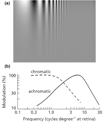
The eye’s ability to detect spatial differences (acuity) depends on the image focused on the retina. In terms of actual spatial features in an image, which may vary over several orders of magnitude, matching one range of frequencies on the ground with the optimum for the eye depends on the scale of the actual images, whether a hard copy print or on a computer monitor. At large scales the finer features show up, such as the surface texture of an outcrop. Reducing the scale and widening the field of view progressively brings into sharp clarity lower spatial frequencies, for instance joints in outcrops, small faults, shadowed topographic features and so on, up to regional variations in brightness patterns due to shadowed relief. With hardcopy that is most easily done at progressively increased viewing distances. At a fixed image scale of 1:S and a viewing distance X m the frequency at the retina f cycles per degree is related to spatial wavelength (the reciprocal of frequency) in the image l m by:
l = S.X.tan(1/f).
As an example, a black and white image at a scale of 1:500 000 viewed from 1 m away gives most visual impact to features that are focused on the retina at 7 cycles per degree (Figure 2.8b). Using the formula, this translates to features with an actual wavelength on the ground of about 1.25 km. Referring to the achromatic plot on Figure 2.8b, features 0.5 and 3.5 km across will excite less than half the visual response, fading for <0.5 and >3.5 km commensurately with the achromatic MTF. Any scene will contain features with a very wide range of spatial frequencies, some of which will have geological or topographic significance. To detect and map them all efficiently requires us to view the scene at a range of scales on a computer monitor, or at a range of distances for a hardcopy image at a fixed scale, bearing in mind the effectiveness of enhanced contrast also revealed by Figure 2.8a. Viewing at a hierarchy of scales is particularly useful in detecting geological structures that may have a bearing on water resources.
Another kind of resolution, which is not so intuitively obvious as that referring to spatial dimensions, concerns the spectral range of EM radiation. Having excellent colour perception, it is easy for us to forget that it is confined to a mere 0.3 micrometres (μm) of the 0.4 to 2.5 μm range of solar radiation that penetrates the atmosphere and is available for remote sensing (Figures 2.2 and 2.3). Examining the spectrum of radiation reflected by a blade of grass over this full range (Figure 2.9) – its reflectance spectrum – it is clear that the reason for it appearing green to us lies in its higher reflectance between 0.5-0.6 μm (visible green) than between 0.4-0.5 μm (blue) and 0.6-0.7 μm (red). The greater absorption of red and blue light than green stems from the pigment chlorophyll. Photosynthesis involves the conversion of water and CO2 to carbohydrates and oxygen in which the chlorophyll molecule exploits the different quantum energies of blue and red radiation to excite electrons in water molecules to split H2O into hydrogen and oxygen.
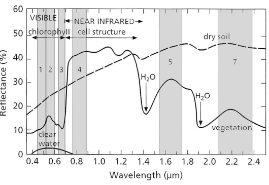
Photosynthesis releases oxygen and uses hydrogen to reduce carbon dioxide to carbohydrates. Yet any substance that appears green to us has much the same spectral features in the visible region, whether it be animal (e.g. a chameleon), vegetable (e.g. grass) or mineral (e.g. malachite Cu2CO3(OH)2). But across the full range of the reflected region photosynthesising vegetation has a unique spectrum (Figure 2.9) that enables it to be unequivocally identified. In fact different kinds of vegetation are sufficiently different from one another for many plants to be identified, given remotely sensed data from several wavelength ranges (referred to as bands from now-on) between 0.4 to 2.5 μm (Figure 2.9). If these bands are positioned strategically relative to the spectral features of different materials and have narrow enough ranges of wavelength to discriminate those features from others, as are bands 4, 3 and 2 in Figure 2.9, it is possible to detect and identify living vegetation. The same principles apply to discriminating between different minerals (Figures 2.12 and 2.13).
The earliest remote sensing by airborne, downward-pointing cameras used photographic film sensitive to all wavelengths between 0.2- 0.7 μm (ultraviolet to red light). The negative ‘black and white’ film used in such aerial photography, properly referred to as panchromatic or ‘pan’, was exposed through a yellow filter to reduce the effect of atmospherically scattered ultraviolet and blue thereby reducing the effect of atmospheric haze. Panchromatic aerial photographs have poor spectral resolution, but reveal details of surface texture and relief shading. They are commonly used in stereoscopic imaging that renders the surface in three dimensions (see Chapter 3) and gives excellent scope for mapping many geological structures, both tectonic and geomorphological.
Colour positive film incorporates three layers of emulsion sensitive to red, green and blue light; the three additive primary colours. When the film has been developed the emulsion retain different proportions of cyan magenta, yellow and dyes respectively (subtractive primary colours), in inverse proportion to the intensities of red, green and blue light that fell on each grain of emulsion, The layers act as filters to white light being passed through thereby reproducing the blend of the three primary additive colours in the photographed scene, and that blend to reproduce the scene in full colour.
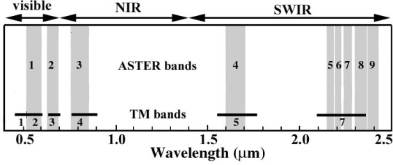
Most photography and all commercial remote sensing in the early 21st century uses digital technology. The most familiar method uses several million charge-coupled devices (CCDs) embedded as a rectangular array in a metal plate, which is the basis for all hand-held digital photography. CCDs combined with filters sense red, green and blue radiation to reproduce the natural colour in the scene. Remote sensing that depends on solar radiation extends the wavelength range that can be detected beyond red into the infrared up to about 2.5 μm, arbitrarily divided into the visible and near infrared (VNIR) between 0.4-1.4 μm and short-wave infrared (SWIR) from 1.4-2.5 μm (Figure 2.9). Using diffraction gratings that direct specific ranges of wavelengths onto individual detectors allows the sensing of specific ‘bands’ of radiation anywhere in the EM spectrum up to the thermal infrared (TIR). The most familiar of such systems to remote sensing scientists is the Thematic Mapper (TM) carried by the Landsat series of satellites, whose 6 reflected band widths (28.5 m spatial resolution) are shown on Figure 2.9. Landsat-7 carried the Advanced Thematic Mapper Plus (ETM+), which also included a thermal infrared band (10.4-12.5 μm) with 60 m spatial resolution and a panchromatic (0.52-0.9 μm) band with 14.25 m spatial resolution. The latest Landsat-8 carries a TM-like system, known as the Optical Land Imager (OLI). Somewhat more advanced is the Advanced Spaceborne Thermal Emission and Reflection Radiometer (ASTER) instrument that senses 4 VNIR bands, 5 in the SWIR and 5 in the TIR (at resolutions of 15, 30 and 90 m respectively. Details of the spectral bands of Landsat and ASTER data, which are used extensively in later chapters and the Exercises, are shown in Table 2.2.
Figure 2.10 compares ASTER bands in the reflected region with those of Landsat ETM+, clearly showing that the spectral resolution of ASTER’s 5 SWIR bands is very much better than the single band 7 of ETM+. So much so that ASTER is able to approximate the spectra of some important minerals present in rocks and soils (Section 2.2.1). The 5 ASTER TIR bands likewise roughly distinguish spectra of some common minerals that emit radiation in different ways at the ambient temperature of the Earth’s surface (Section 2.2.1).
The most spectrally revealing kind of remote sensing divides up and senses the whole reflected and thermally emitted regions as many narrow bands, with spectral resolutions of the order of 10 nm or less in the reflected region and 30-70 nm for thermal emission. Such hyperspectral imaging systems are able to produce spectra of surface materials that are comparable with those produced under laboratory conditions. However, only one such system has been deployed in Earth orbit (NASA’s EO-1 Hyperion), although several are deployed around the Moon, Mars and Mercury (e.g. OMEGA carries by the European Space Agency’s Mars Express; CRISM carried by NASA’s Mars Reconnaissance Orbiter). Ironically, the rest of the Solar System is better served by orbital remote sensing than is the Earth as regards spectral and spatial resolution, and affordability of the data: high spatial resolution terrestrial data from orbit, and all airborne digital imagery is extremely costly (US$5-25 km-2; Appendix 1).
2.2 Matter and EM radiation
When EM radiation meets a material the radiant energy is conserved at all wavelengths so that the incoming radiant energy at one wavelength (EI)λ is distributed between reflected (ER)λ, absorbed (EA)λ and transmitted energy (ET)λ, so that:
(EI)λ= (ER)λ + (EA)λ+ (ET)λ
Dividing all the terms in the equation by the incoming radiant energy (EI)λ produces an expression that defines the spectral properties of the material as three ratios: (ER/EI)λ, (EA/EI)λ and (ET/EI)λ, whose values are called the spectral reflectance (ρλ), absorptance (αλ) and transmittance (τλ) respectively, so that:
ρλ + αλ + τλ = 1
Most geologically important minerals and rocks are opaque except in thin section, so that their transmittance is zero, and that equation reduces to:
ρλ + αλ =1; or αλ – 1 = ρλ; or ρλ = 1 – αλ
Plant leaves and water transmit radiant energy to some extent. In the VNIR and microwave (radar) regions of the EM spectrum remote sensing relies on the energy reflected by a material.
How a material reflects energy depends on its roughness relative to the wavelength of radiation. If a surface is relatively smooth, it behaves in a mirror-like or specular fashion (Figure 2.11a) so that all reflected energy is directed away from it at the same angle as incoming falls on it. A relatively rough surface has facets that are randomly oriented in relation to the direction of illumination and reflection tends to be diffused in all directions (Figure 2.11b), although most natural surfaces produce a specular component too (Figure 2.11c). Unless highly polished and mirror-like, natural surfaces are extremely rough relative to the wavelengths of VNIR and SWIR radiation, so reflection from them is dominantly diffuse in all directions.
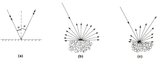
Interestingly, the wavelengths used in radar remote sensing (between 1 cm and 1 m, Table 2.1) are comparable with the roughness range of most natural surfaces. Depending on radar wavelength, those surfaces that have surface relief below a certain range of dimensions reflect all microwave energy almost perfectly. Since radar images are produced by energy directed obliquely sideways towards the Earth’s surface, such ‘radar smooth’ surfaces reflect all energy away from the receiving antenna, and so appear black on the radar image. Rougher surfaces relative to radar wavelength produce diffuse reflections, so that some of the energy does return to the antenna: in radar parlance, that is called backscatter. Exploiting the two orders of magnitude differences in radar wavelengths therefore enable surfaces with different textures to be discriminated in terms of their ‘radar roughness’. Interestingly, if an object has three flat surfaces, such as joint surfaces in a rock outcrop, arranged at right angles, when radar energy hits one rectangular facet, it is reflected to the others, which also reflect the radar. Consequently, most of the energy eventually returns directly to the antenna giving a much more intense signal than that from normal backscatter. This is the principle used in the ‘corner reflectors’ placed on the masts of ships so that they are easily detected by the radar of other vessels, even if the ship itself is wooden or quite small. Such a complete reflection appears as a star-like feature or ‘bloom’ on a radar image (for more detail on radar remote sensing, see Chapter 4, Section 4.2).
2.2.1 Reflectance and emittance spectra
The important thing about reflectance spectra and using them to identify minerals is not the ability of a material to reflect radiation, but rather its ability to absorb EM energy over often distinctive ranges of wavelength. The underlying principle is quantum theory, as outlined earlier to explain the green colour of grass to human vision. At the molecular, atomic and sub-atomic levels changes in the structure and behaviour of matter require energy in discrete amounts or quanta. Electromagnetic radiation behaves as photons that link electric and magnetic force fields and which travel at light speed. The energy (E) carried by photons varies in inverse proportion to the wavelength of radiation, expressed by Planck’s Law:
E = ch/λ,
where c is the speed of light, h is Planck’s constant (6.62 x 10⁻³⁴ J s) and λ is wavelength.
Consequently, the shorter the wavelength of radiation, the more energy is carried by each photon. One outcome of this is connected to the resolution of detectors. A detector, such as a CCD, requires a particular energy to produce a measurable response; the shorter the wavelength being detected the less photons are needed to give a response. As a result, as wavelength increases, in order to respond the detector either has to be bigger or has to be exposed to radiation for longer. In both cases this reduces the spatial and spectral resolving capacity for longer wavelengths. In practice the choice is a trade-off between the two kinds of resolution: to increase spatial resolution requires detection of a wider range of wavelengths; to increase spectral resolution demands larger detectors and decreased spatial resolution. The ASTER system expresses this neatly: its 5 SWIR detectors allow bands to be 0.04 μm wide at a spatial resolution of 30 m, whereas its 5 TIR detectors produce spectral bands 10 to 20 times wider at 90 m resolution.
A more important feature stemming from the quantisation of EM energy is absorption of specific wavelengths by shifts in the behaviour of matter. Every chemical element can exist in several possible states according to: the nature of the bonds in which it participates; its position in a molecule in relation to atoms of other elements; the energy levels of its outermost electrons and a great deal more. To understand the spectra of materials for practical remote sensing a grossly simplified account is quite adequate. For an electron, an atom or a bond in a molecule to shift from one quantum state to another – to undergo a transition – requires energy, delivered by photons in the case of remote sensing. For an outer-shell electron to be excited from its ground state to a higher orbital requires a specific amount of energy. This results in absorption of photons of the appropriate wavelength, and because the quantum energy needed is high those photons are of short wavelength. Elements that exhibit such electronic transitions best are those with several possible valence states, such as iron, manganese and chromium. The absorptions take place in the visible part of the EM spectrum, where quantum energies are high, and therefore impart colour to compounds of these elements, the most important of which at the Earth’s surface are rock-forming minerals, such as the silicates. However, because rocks and the minerals in them are weathered to more stable breakdown products and often contain impurities the green colour of olivine, for instance, does not show up in natural outcrops.
Of the main rock-forming minerals only quartz and carbonates are not broken down to other minerals by weathering, although both may be dissolved under certain conditions. There are a few silicate minerals that may remain fresh for long periods of weathering: chlorites, epidote and white micas that are common in metamorphic rocks derived from mafic igneous rocks or impure clays. Feldspars – anhydrous aluminosilicates of K, Na and Ca – weather to clay minerals and soluble ions of the alkali- and alkaline-earth metals. Ferromagnesian silicates – biotite mica, amphiboles, pyroxenes and olivines, plus many iron- and magnesium-rich metamorphic minerals – break down to clays, insoluble iron-3 oxides and hydroxides, plus soluble Mg and other ions. Except in the most arid or cold conditions or where physical weathering continually exposes fresh surfaces, the outermost few micrometres of exposed minerals are dominated by their solid weathering products. For EM wavelengths in the VNIR to SWIR range, most of the energy detected by remote sensing emerges from that thin rind. Its variation with wavelength, up to 2.5 mm, is mainly determined by the iron oxides and hydroxides, clays, a few resistant iron-rich phyllosilicates, and different proportions of quartz and carbonates that make up most of the weathered veneer. These can be conveniently considered by grouping them as dark- and light-coloured minerals.
Dark-coloured minerals that are likely to be preserved in soils and the weathering veneers of rock outcrops are dominated by the common oxides, hydroxides and sulfates of Fe-3 produced by weathering: hematite (Fe2O3), goethite (FeOOH) and jarosite (KFe3+3(OH)6(SO4)2). In powdered form, as thin veneers of weathered surfaces or coatings on grains of other minerals, these appear red, brownish and orange respectively. Their spectral features in the VNIR (Figure 2.12a) show why we see them in such colours. Outer-shell electrons in iron atoms are sufficiently energetic that they can be transferred from one atom to another, giving a certain level of electrical conductivity to the three minerals. The quantum energy needed to achieve such a charge-transfer transition is available from photons in the green to blue range, resulting in a broad absorption that leaves red wavelengths to be reflected more strongly.
In the near infrared the three iron minerals in Figure 2.12a exhibit another strong and characteristic absorption. All three are ionic compounds in which the component cations and anions are held together by an electrostatic field. The relationships between negatively charged anions (e.g. oxygen) surrounding positively charged cations (especially of transition metals such as iron) distort the electric field in the crystal, according to mineral structure. This crystal field effect changes the energies that move electrons to different levels in orbital shells.

The coloured minerals chlorite and epidote are common in low-grade metamorphic rocks, biotite characterising many higher grade schists. All three are moderately resistant to chemical weathering. The medium- to high-grade metamorphic equivalent of basalt is amphibolite, in which all iron and magnesium plus some calcium is contained in amphiboles. The dark colour of these mineral to our vision stems from their low reflectance in the visible range (Figure 2.12b). However, it is in the infrared that these minerals become most spectrally distinctive. Their reflectances rise to the highest levels in the SWIR range, which also includes very distinctive absorptions, due to stretching or bending of simple Mg-OH and Fe-OH bonds in their structure – vibrational transitions. Each distortion requires a narrow range of energies that can be supplied by EM photons
Among the light-coloured minerals, quartz shows no absorption features at all in the VNIR to SWIR region to produce a flat spectrum (Figure 2.12c). However, quartz is highly reflective in all wavelengths, and has a high albedo, so it imparts a bright signature to rocks and soils in which it is abundant. For much of the visible to SWIR range so too do carbonates and clays, but they have distinctive absorption features due to vibrational transitions. Stretching and bending of the C–O bond of CO32- in the ionic crystals of carbonates are achieved by quantum energies carried by photons around 2.3 mm (Figure 2.12c). The other common bright minerals are clays, but they have several absorption features (Figure 2.12c). Most obvious are those that stem from stretching and bending of the H–O–H bonds in the water that all clays contain, occurring at around 1.4 and 1.9 mm. More important are their absorptions around 2.15-2.21 mm that are due to stretching of the Al-OH bond in the structure of clays, which they share with muscovite (white mica) (Figure 2.12c). Montmorillonite, illite and kaolinite clays are each subtly different, notably kaolinite that has two overlapping absorptions at 2.16 and 2.21 mm. The oddities among clays are those like saponite that have magnesium in their structure having formed by weathering of olivine in ultramafic rocks. They show an absorption feature at 2.315 mm related to distortion of the Mg-OH bond in their structure, similar to ferromagnesian silicates (Figure 2.12b).
Important electronic transitions for remote sensing are those associated with the plant pigment chlorophyll (Figure 2.9), of which there are several types. Chlorophyll molecules (e.g. C55H72O5N4Mg) are ‘tadpole-shaped’ with ‘heads’ that centre on magnesium and tails that combine C, H and O and have the peculiar property of double absorption because of electron excitation. That in the blue part of visible light excites electrons in water molecules of the plant cell, which oxidise water to oxygen and hydrogen ions, the lost electrons being taken up by chlorophyll. The other absorption in the red further excites electrons in chlorophyll itself, which help in the reduction of carbon dioxide by its combination with hydrogen ions that lies at the root of photosynthesis of carbohydrate and free oxygen. The whole is expressed by
CO2 + H2O + e– = (CH2O) + O2,
although it is a great deal more complex chemically. Various other plant pigments employ similar electronic transitions, such as those that impart reddish and brownish colours to seaweeds through absorptions in blue and green. Because there are several forms of chlorophyll that absorb at slightly different wavelengths, the net result is two broad absorption features (Figure 2.13) that give chlorophyll and most plants their green coloration. But being green is obviously not an exclusive feature of plants.
Plants are truly unique in the wavelength range just longer than visible red, as a result of an evolutionary process in their cells. Photosynthetic pigments break down above about 70º C, as do plant cells, to result in wilting. All solar energy absorbed by materials serves to increase their temperature. To avoid such heating plants have evolved a degree of transparency so that all wavelengths pass through them to some extent, and shiny coatings that reflect a proportion from the surface.

More important for remote sensing are cell structures that produce efficient internal refraction and reflection of wavelengths longer than visible red to give the leaves of most plants a strong reflectance peak between 0.7 to 1.3 μm (Figure 2.9). Reflectance rises sharply at wavelengths just greater than visible red to give rise to the red-edge effect. The shape of this feature depends upon the type of vegetation (Figure 2.13a), sufficiently for different species to be discriminated. Moreover, spectra of vegetation change with the seasons as their pigmentation changes with autumnal senescence or with water stress (Figure 2.13b). At longer infrared wavelengths, spectral of plants show two strong absorption features at ~1.4 and 1.9 μm due to water in the cell structure (also seen in minerals that contain molecularly bound water of water in fluid inclusions – Figures 2.9 and 2.12c). As plants experience shortages of soil moisture, these features become shallower and the overall reflectance or albedo of leaves increases (Figure 2.13b). The red edge and shifts in the overall shape of vegetation spectra can be addressed by image processing to develop graphic measures of vegetation density, water stress and disease (Section 2.2).
Water has unique properties in the VNIR to SWIR range due to both transmission and absorption. In the visible range transmission through clear water less than ~40 m deep allows a proportion of solar energy to reach the bed and be reflected back, the penetration depth increasing as wavelength decreases so that blue radiation only is reflected back by water that is more than 40 m deep. It is therefore possible to estimate depth in shallow, clear water from the intensity of light reflected from the bed. To some extent water takes on the spectral properties of material suspended in it, such as sediment or plankton. However, beyond visible red, water absorbs all solar wavelengths and therefore appears black on near- and short-wavelength infrared images. There are minerals, such as sulfides, manganese oxides and hydroxides, and carbon derived from decayed organic matter, which have very low reflectance and appear black in all reflected wavelengths, as do areas of deep shadow. So water is not unique in its appearance on VNIR and SWIR images, but can be distinguished easily from other dark features by occupying narrow meandering channels and sharply defined lakes.
The theory of how radiation is emitted by materials stems from the concept of a blackbody: a perfect emitter that obeys the Stefan-Boltzmann and Wien’s Displacement Laws, as expressed by Figure 2.1. In reality the only material that approaches a blackbody is water, which enables surface water temperatures to be estimated from thermally emitted data – the effects of evaporative cooling and the atmosphere do not permit exact calculations of, say, sea surface temperatures. All other materials deviate markedly from blackbody behaviour in one way or another, exemplified by Figure 2.14 showing the emissive properties of the most common inorganic material on the land surface, quartz, relative to those of a perfect blackbody.
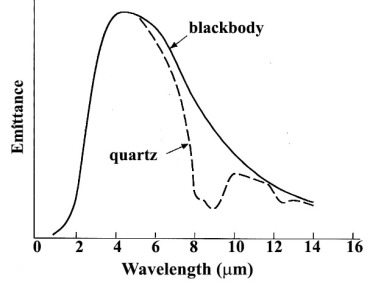
The marked trough in the emission spectrum of quartz between 8 to 10 μm results from thermal energy being used to stretch the Si-O bond in the SiO2 molecule of quartz. The Si-O vibrational transition occurs in all silicate minerals, but its wavelength range varies markedly according to their specific molecular structure, which affects how the SiO4 tetrahedral ‘building blocks’ of all silicates share oxygen atoms (Figure 2.15). Similar restrahlen bands characterise carbonates (C-O bond stretching) and clay minerals (Si-O-Si) (Figure 2.15). Iron oxides and hydroxides tend to show uniformly high emission in featureless spectra. Most living vegetation has low daytime thermal emission due to the cooling effect of evapotranspiration and appears dark in all ASTER TIR bands. So TIR data relate specifically to many rock-forming minerals in igneous, sedimentary and metamorphic rocks. An important aspect of thermal emission from rocks and soils is that it emerges from the outer few centimetres of their surfaces, rather than a few micrometres in the case of reflected radiation. As a result, TIR data are less affected by superficial veneers of weathered material.

2.2.2 Spectral coverage of free and low-cost satellite image data
Chapters 4 and 5, and Exercises 1 to 4 mainly refer to images from two systems: Landsat, L-4 and -5 carrying the multispectral Thematic Mapper (TM), L-7 the Enhanced Thematic Mapper+ (ETM+) and L-8 the Operational Land Imager (OLI), data from which are free per 185 x 170 km scene; the Advanced Spaceborne Thermal Emission and Reflection Radiometer (ASTER) carried by the NASA Terra and Aqua satellites, data from which are free per 60 x 60 km scene. Table 2.2 shows the wavelength ranges of the detectors deployed by these instruments.
Table 2.2 Details of Landsat and ASTER data (* – panchromatic bands; † – for high cloud detection; ‡ stereo bands 3N and 3B.
| Landsat-7 ETM+ Landsat-4 & -5 TM (bands 1-7 only) | Landsat-8 OLI | Terra ASTER (VNIR & SWIR) | Terra ASTER (TIR) | ||||
| Band | Range (µm) | Band | Range (µm) | Band | Range (µm) | Band | Range (µm) |
| 1 (28.5) | 0.45-0.52 | 1 (30) | 0.44-0.45 | 1 (15) | 0.52-0.60 | 10 (90) | 8.13-8.48 |
| 2 (28.5) | 0.52-0.60 | 2 (30) | 0.45-0.51 | 2 (15) | 0.63-0.69 | 11 (90) | 8.48-8.83 |
| 3 (28.5) | 0.63-0.69 | 3 (30) | 0.53-0.59 | 3 (15) | ‡0.76-0.86 | 12 (90) | 8.93-9.28 |
| 4 (28.5) | 0.76-0.90 | 4 (30) | 0.64-0.67 | 4 (30) | 1.60-1.70 | 13 (90) | 10.25-10.95 |
| 5 (28.5) | 1.55-1.75 | 5 (30) | 0.85-0.88 | 5 (30) | 2.145-2.185 | 14 (90) | 10.95-11.65 |
| 6 (60) | 10.3-12.4 | 6 (30) | 1.57-1.65 | 6 (30) | 2.185-2.225 | ||
| 7 (28.5) | 2.08-2.35 | 7 (30) | 2.11-2.29 | 7 (30) | 1.235-2.285 | ||
| 8* (14.5) | 0.52-0.90 | 8* (15) | 0.50-0.68 | 8 (30) | 2.295-2.365 | ||
| 9† (30) | 1.36-1.38 | 9 (30) | 2.36-2.43 | ||||
| 10 (100) | 10.6-11.2 | ||||||
| 11 (100) | 11.5-12.5 | ||||||
Chapter 5 concentrates on how various combinations of band data from these instruments can be used to highlight, discriminate and detect various surface materials, principally minerals rocks and bare soils. Appendix 1 shows how to obtain data from the principal data archives.
If you found this Chapter useful you may wish to download all chapters as an eBook, which may be more convenient for future reading
Useful References
Andrews Deller, M.E. 2006. Facies discrimination in laterites using remotely sensed data, International Journal of Remote Sensing, 27, 2389–2409.
Drury, S.A., 2001, Image Interpretation in Geology, (3rd edition) Nelson Thorne/Blackwell Science: London. [Includes image processing course on CD-ROM]
Liu, J.G. & Mason, P.J. 2016. Image Processing and GIS for Remote Sensing : Techniques and Applications. John Wiley & Sons: Oxford.
Prost, G.L. 2013. Remote Sensing for Geoscientists: Image Analysis and Integration, (3rd edition). CRC Press
Short, N. 1999. The Remote Sensing Tutorial. Federation of American Scientists; online resource. [Comprehensive guide to all aspects of remote sensing; patchy quality]
Vincent, R.K., 1997, Image Fundamentals of Geological and Environmental Remote Sensing, (2nd edition). Prentice Hall: New Jersey.
